F5 Data: A Swiss Army Knife for Storm Chasers Adds Some Superb New Tools

I first began using F5 Data in 2007, and despite its early developmental quirks and my own vast lack of experience at forecasting, I fell in love with it. Storm chaser and program designer Andrew Revering had a solid and unique concept, one that gave me an ample tool for both learning forecasting and chasing storms. In particular, its configurable overlay of RUC maps on top of my GR3 radar images (via Allisonhouse’s data feed) appealed to me. At a glance, I could get a good idea of the kind of environment storms were moving through and into. And I had more than 160 parameters to choose from. I hadn’t an inkling what most of them were for, but they were available to me if ever I learned.

In 2008, Andy made significant upgrades to his product with the addition of color shading and contouring, GFS at 3-hour intervals out to 180 hours, a calculator for instantly converting various units of measurement to other units of measurement ( such as meters per second to knots and miles per hour), and other improvements.  The result not only looked attractive and professional, but it offered more solid bang for the buck–and at a little over $14.00 a month, the bucks were easily affordable.

Map Overlays: An Immensely Useful Feature

500 mb Heights

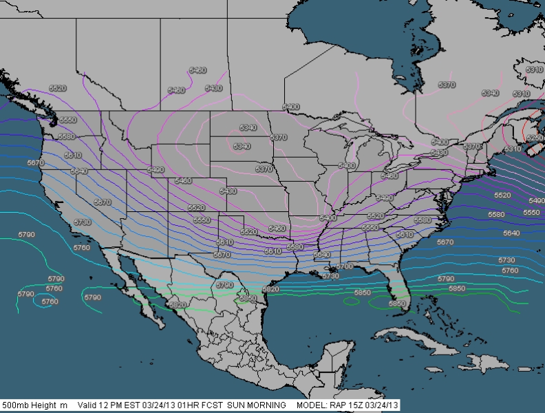
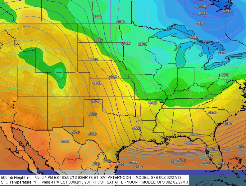
CONUS view showing 500 mb height contours. Note: Images shown here do not correspond to the text example.

At the same time, my own forecasting skills were slowly improving, and as they did, I came to greatly value another key feature of F5 Data: its ability to layer any of its maps on top of each other. This is a hugely useful feature and one I haven’t seen in any other commonly available forecasting resource that doesn’t require more technical skills than I possess. F5 Data is easy and intuitive to use, and as my knowledge grew, so did my appreciation for its map overlays.

F5 Sample Overlays

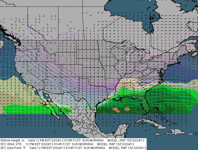
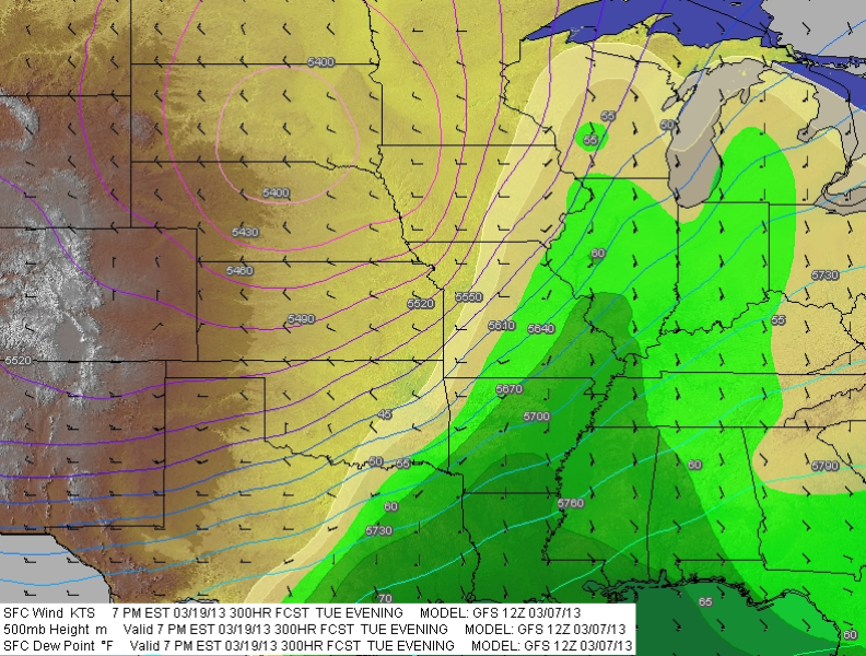
CONUS view with shaded surface dewpoints and surface wind barbs added to 500 mb heights contours. Labels for dewpoints have been turned off.

F5 Overlays Zoomed

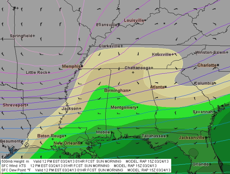
Same overlays as above zoomed in to selected area.

Say, for instance, I’m looking at the NAM 48-hour forecast for 21Z. I select the 500 mb heights map, choosing the contour setting, and see a trough digging into New Mexico, with diffluence fanning across the Texas/Oklahoma panhandles up into Kansas. How is the boundary layer responding? Switching from contours to shading, I select sea level pressure, and now, superimposed on the H5 heights, I can see a 998 mb low centered in southwest Kansas. Another click adds surface wind barbs, which show a good southeasterly flow toward the low, with an easterly shift across northern Kansas suggesting the location of the warm front. Hmmm, what’s happening with moisture? Deleting the SLP map–I don’t have to, but too many maps creates clutter–I select surface dewpoints. Ah! There’s a nice, broad lobe of 65 degree Tds stretching as far north as Hutchinson, with a dryline dropping south from near Dodge City into Oklahoma and Texas. Another click gives me an overlay of 850 mb dewpoints, revealing that moisture is ample and deep. Still another click shows a 70 knot 500 mb jet core nosing in toward the panhandles.

You get the idea. I can continue to add and subtract maps of all kinds–surface and mixed-layer CAPE, 3 km and 1 km storm-relative helicity, bulk shear, 850 mb wind speed and directional barbs, EHI, STP, moisture convergence, and whatever else I need to satisfy my curiosity about how the system could play out two days hence. I can see at a glance favorable juxtapositions of shear, moisture, lift, and instability per NAM. And I can make similar comparisons with GFS, and on day one, with RAP (which replaced RUC in May 2012).

And Now the Upgrade: Presenting Version 2.6

Everything I’ve written so far has been to set a context for what follows, which is my review of the latest major upgrade to F5 Data. It comess at a time when the number of forecasting products available online has greatly expanded and old standbys have updated in ways that make them marvelously functional. Notably, a number of years ago TwisterData gained rapid and massive acceptance among storm chasers, and it continues to enjoy prominence as a quick, one-stop resource. Like F5 Data, it features GFS, NAM, and RAP, and it also offers point-and-click model soundings, a very handy feature. In 2010, the HRRR brought hourly high-resolution maps to the fray, with its forecast radar images demonstrating considerable accuracy. And the SPC’s Mesoanalysis Graphics, always a stellar chase-day resource, has recently made some dynamite improvements. Today the Internet is a veritable candy store of free forecasting resources.

GR3 with F5 mesoanalysis overlay. This one shows surface and 850 mb Tds and 850 wind barbs. (The blue wind barbs are an Allisonhouse product.)

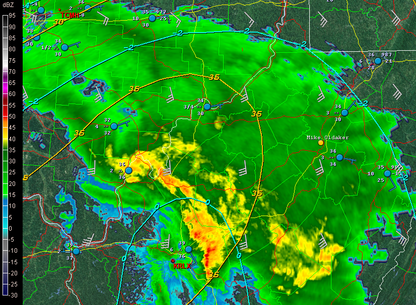
GR3 with F5 mesoanalysis overlay. This one shows surface and 850 mb dewpoints and 850 mb wind barbs. (The blue METARs are an Allisonhouse product.)

At the same time, F5 Data didn’t seem to be doing much, and while I still resorted to it constantly, I wondered whether Andy had lost his passion and commitment to his product. Most troubling to me, the proprietary mesoanalysis maps which had replaced the RUC maps as GR3 overlays often failed to update in a timely manner, rendering them pointless. Given their potential usefulness in the field–how valuable would it be, for instance, to see at a glance that the storm you’re following is moving into greater instability and bulk shear?–I found this disappointing.

But I no longer have any such concerns. This latest upgrade has rendered F5 Data a powerhouse. All the while, Andy was beavering away in the background, fixing bugs and incorporating various client requests into his own set of huge improvements to his creation. Beginning with the February 1, 2013, release of v. 2.5 and moving in seven-league strides toward the latest version, 2.6.1, these changes have been a long time coming, they reflect a lot of work on Andy’s part, and they have been well worth the wait.

Here’s What Is New

The following will give you a quick idea of the more significant changes:

  • NAVGEM has been added to the F5 suite of forecast models.
  • Users can now draw boundaries, highs, and lows.
  • Users can select increments other than the default by which arrow keys advance forecast hours for the different models
  • The map now offers an experimental curved-Earth projection.
  • Wind barbs at different levels can be overlaid to provide visuals of speed and directional shear.
  • Processing is faster (up to 45 minutes faster with GFS)
  • Text for geographic maps can now be customized.

And yes, the mesoanalysis maps are now on the money. Andy moved them to a faster server, and they now update regularly and consistently, to the point where I plan to display some of them on my site the way I used to do with the F5 Data RUC maps.

All of the above are in addition to the already existing array of features. A few of these include the following:

  • Over 160 parameters, including ones you just don’t find elsewhere, such as the Stensrud Tornado Risk and isentropic surfaces, and also a good number of proprietary products such as the APRWX Tornado Index, APRWX Severe Index, and APRWX Cap.
  • Current conditions plus five forecast models: GFS (out to 384 hours), NAM, RAP, hourly mesoanalysis, and the newly added NAVGEM.
  • Mesoanalysis integration with radar products via Allisonhouse (already described).
  • A point-and-click CONUS grid of forecast soundings.
  • Zoom capabilities that let you zero in on areas of interest. Activate the display of cities and roads and target selection gets that much easier.
  • National satellite (visible, water vapor, and infrared) and base reflectivity radar composites.
  • Fully customizable map overlays (as discussed above).
  • 14 categories of maps organized for particular purposes, including Severe, Tornado, Hurricane, Cold Core, Winter, Lift, Shear, and Moisture. These are fully customizable, and you can create your own categories if you wish.
  • Watch and warning boxes.

To describe all of the features that F5 Data offers would take too much space and isn’t necessary. You can find out more at the F5 Data website, which includes a whole library of video tutorials on what F5 Data is and how to use it.

Better yet, you can download the software (it’s free) and try it out for yourself with 17 free maps.

If there is any downside to the upgraded F5 Data, it is minor and purely personal. I miss the passing of the historical data feature some months prior to the main upgrade. That feature allowed me to request data for past forecast dates and hours so I could study chase setups from years gone by. I wish I still had that option. However, I understand that it needed to go in order for Andy to move ahead with his changes. The feature was peripheral to the purpose of F5 Data, evidently it didn’t get used much, and it’s a small price to pay for the big improvements to this forecasting resource.

One thing Andy might consider for a future update would be to break down SBCAPE and MLCAPE contours into smaller increments. CAPE is displayed by intervals of 100 from 0–500 J/kg, which is great; but from 500 up to 3,000, it jumps by units of 500 J/kg, and from 3,000 on up it moves 1,000 J/kg at a time. Realistically, these are just overviews of instability, and they’re in keeping with how most other forecast resources display CAPE. If you want to get more granular, you can always check out forecast soundings. Still, it’s an opportunity for F5 Data to provide a somewhat more incremental breakdown similar to that of TwisterData.

With these last two comments dispensed of, I highly recommend to you the new and improved F5 Data. It’s easy to use and flexible as all getout, and it puts a squadron of tools at your disposal, all in one eye-pleasing, zoomable interface. Of course, no one forecasting resource covers all the bases, and that is certainly true of F5 Data. But this is nonetheless a fabulous product that offers some unique advantages. These latest changes, including the addition of NAVGEM, the ability to draw boundaries, and mesoanalysis graphics that update regularly to provide the most current information, have taken an already fine resource and made it dramatically more useful.

Bravo, Andrew Revering! You do great work.

This review, by the way, is unsolicited and unpaid-for. I’ve been a fan of F5 Data and of Andy from the start, and I’m pleased to share my thoughts about the latest iteration of a product I’ve used extensively and benefited from for a good number of years.


The Foibles of Long-Range Forecast Models

Tues_March_19_GFS300hrsSometimes a picture really is worth a whole lot of words. In this case, two tell the story more eloquently than I can.

In the image to your left, the 12Z run of the  GFS depicts 500 mb height contours, surface moisture, and surface winds at 300 hours out, or twelve days before the forecast date.

The second image, taken just a little while ago, shows the same information for the same system, only now we’re down to just 66 hours from forecast time. Note that the forecast date has moved up a day to Monday; by Tuesday, the whole system has moved off to the east and out to sea. Bye-bye moisture and instability.

Mon_March_18_GFS66hrsWhat happened? The GFS happened, that’s what.

I realize that for many of my storm chasing readers, maybe most of you, I’m preaching to the choir, but some may wish to take note of the following:

Long-range forecast models are notoriously undependable and prone to change.

If you’ve never heard the colloquialism wish-casting, now’s the time to add it to your storm chasing lexicon. The further out you go beyond three days from an event, the more that attempting to forecast a chaseable setup amounts to just a hope and a prayer. Bad data and changing data amplify progressively in the numerical models, to the point where what you see at 240 hours out is subject to anything from mild to wild fluctuation and revision as the forecast hour draws closer and new data gets processed. By the time the NAM and SREF lean in, and finally the RAP and HRRR, what you see may resemble nothing like the deep, negatively tilted trough and gorgeous moisture plume that first captured your attention. The shape, the timing, wind speed and direction at different heights, quality of moisture, instability–everything can change, and it will, possibly quite drastically.

Remember the gossip chain? Anna tells Peter, “Selena just bought a used Nissan from the same car dealer where Jaden bought his truck. It’s on 44th Street about a mile from the dump.” Peter passes the news on to Sam thus: “Selena just bought a car from the same dealer where Jaden got his truck next to the 44th Street dump.” Sam tells Chelsea, and Chelsea tells Adam, and so it goes, with the information getting nuanced a little more each time until it becomes outright twisted. Finally, word gets back to Selena: “Hey, Selena, what’s this I hear about you buying the dump over on 44th Street from some drug dealer?”

It can be kind of that way with long-range forecasts.

So why even bother watching the long-range models, particularly the famously untrustworthy GFS? There are two reasons. One is, the models can provide a heads-up to the possibility of a chaseworthy setup. At 192 hours out, don’t think of the models as forecasts–think of them as potential forecasts, something to keep an eye on. A given scenario could fall completely apart and often does. But it could also develop run-to-run consistency that agrees with the short-range models as they enter the picture, and ultimately lead to a decent chase.

For those of us who have to drive a long distance to Tornado Alley, such advance awareness is particularly valuable. If you live in Chickasha, Oklahoma, or Wichita, Kansas, you can roll out of bed in the morning, look at the satellite, surface obs, NAM, and RAP, and decide whether you’re going to chase in the afternoon. But if you live in Grand Rapids, Michigan, or Punxatawney, Pennsylvania, things aren’t that easy. When you’ve got to travel 800 to 1,000 miles or more to get to the action, burning time and fuel and perhaps vacation days, lead-time becomes important, and the more, the better.

The second reason for watching the long-range models is sheer obsessiveness. Call it desperation if you wish. It has been a long winter and storm chasers are itching to hit the road. Some of us just can’t help ourselves–we want to see some flicker of life, some sign of hope, some indication of the Gulf conveyor opening for business beneath a warming sun and dangerous dynamics. What’s the harm in that? Most of us know enough not to hang our hats on a 120-hour forecast, let alone one that’s two weeks out. But it doesn’t hurt to dream. After all, sometimes dreams come true.

Remembering the Henryville EF4 Tornado: A One-Year Retrospective

We were three-and-a-half miles north of Palmyra, Indiana, when the tornado crossed the road less than a mile in front of us at Dutch Creek Road, ripping up a 12 x 12-foot section of asphalt in the process and throwing it in chunks into an adjacent field. Within about a minute, the vortex had morphed from a wispy rope into a powerhouse of a stovepipe, tearing tangentially across our path as Bill Oosterbaan and I blasted north on State Road 135.

Bill is no timid driver, and he did a heck of a job keeping pace with the beast. But the storm was a missile, moving at least 60 miles an hour, and once we hit downed power lines at Dutch Creek Road, we had to let it go. We had no idea of the tragedy it was about to inflict to our northeast. But, watching the white condensation funnel billow and intensify beyond the treeline, with secondary vortices wrapping around it like a cloak, we could tell it was a monster. As I filed a report on Spotter Network, Bill turned around and headed back south. A second supercell was hot on the heels of the one we had just let go, and repositioning became our immediate concern.

Bill and I had just been fortunate to catch and videotape the Henryille EF4 tornado in its formative stages. We first glimpsed it south of Palmyra as it descended from a wall cloud several miles to our west-northwest. It didn’t look particularly impressive at that point, but as we closed in, the fast-moving circulation began to display wild shapes and motions, then condensed fully and finally just before crossing the highway.

It seems incredible that  in the few meager seconds the tornado took to translate across SR 135, it managed to rip up a large section of road. The term “asphalt scouring” just doesn’t apply; there was no scouring involved. An estimated 10,000 pounds of pavement got literally torn from the downwind side of the highway and thrown something like one hundred feet. I didn’t witness this road damage and only found out about it later. But chaser Simon Brewer provides a good description of what he saw just a few-score yards north of where Bill and I turned around.

The wider damage path associated with the main tornado circulation was easily visible from a forest west of the highway through a field, and past the highway through another forest to the east. Also, an individual suction vortex damage path was easily found starting in the field scouring vegetation and tossing boulders from a drainage ditch, then crossing a section of highway peeling and tossing massive slabs of asphalt, the largest broke upon second contact with the ground (it bounced leaving an significant impact crater) on the downwind side of the highway. Typical sphalt scouring is usually associated with EF3 and stronger tornadoes, but typical asphalt scouring is found on rural roads with relatively thin asphalt 1-2 inches or less thick. It’s amazing to think how short a time period the small suction vortex was probably over that section of highway; maybe only a second tops! I usually don’t stop to investigate tornado damage, but when I saw the highway damage on March 2nd I was blown away! I took more photos of the road damage than I did the storm and tornado. I consulted Dr. Greg Forbes and he agreed this was one of the most incredible damage cases he’s heard, only possibly being eclipsed by the trench created by the Philadelphia MS EF5 on April 27, 2011.*

A year has passed since all of the above took place. At the same time last year as I am presently writing these words, Bill and I were nearing Louisville, and within another hour or so we would shift into chase mode, head west, and intercept our storm. Click here to read my complete account of that chase, including my video of the tornado as well as radar images and skew-Ts.

Today the weather is drastically different. This March is behaving like March, not May, and in light of last year’s prolonged heat wave and disastrous drought, I am glad. I will be delighted to see another round or two of good winter weather bring still more moisture to the Plains and Midwest and prime the pump for storm season. The storms of spring will get here soon enough, and while nothing is certain, my hunch is that this year will be better than last year.

_______________

* Simon Brewer, from his January 14, 2013, post in the Stormtrack thread The EF Scale and Asphalt Scouring Caused by the March 2 Henryville Tornado. Also see Simon’s and Jim Bishop’s chase account, which includes photos of the road damage, at their Stormgasm website. You can see Dutch Creek Road just past the road sign and parked car in the background of the first photo.

Enter March: No Repeat of 2012

March 2 2013 GFSMarch 2013 won’t be making anything like last year’s brutal grand entry. For residents of the Ohio valley, that is a good thing. On March 2 a year ago, unseasonably springlike conditions fostered an outbreak of tornadoes, including the violent Henryville, Indiana, tornado that my friend Bill Oosterbaan and I intercepted north of Palmyra.

This March’s arrival portends nothing like that. One look at the map (click to enlarge) will show you that conditions are quite different from last year. The model is today’s (February 27, 2013) 00Z run showing the 500 mb heights and surface temperatures for March 2 at 21Z. With a ridge dominating the western half of the CONUS and cold Canadian air sitting atop the Great Lakes, the picture doesn’t even remotely resemble the 2012 scenario that sent storm chasers scrambling for their gear. A few days prior to the event–that is, right about now–we were casting anxious eyes on the embryonic system with the sense that northern Dixie Alley was in for it.

I’m frankly glad that a cooler, more quiescent opener is in store for the 2013 meteorological spring. I will be pleased to get more snow, and I hope the Midwest and Great Plains get a few more good, solid dumpings before storm season arrives in earnest. Storm chasing aside, the more moisture, the better for regions that have languished under severe drought. As inconvenient as the recent blizzard was for west Texas, I’ll bet the folks in Amarillo were mighty glad to get that much snow. I hope they get more, or just water in abundance in whatever form it takes.

This March may be entering on the cold side, at least here in Michigan, but that’s okay. It is March, the month of transition. I’m equipped with a “new” used car, a 2002 Toyota Camry that is drum tight and ready to take me wherever I need to go in order to see tornadoes. It won’t be long now. See y’all under the meso!

Gulf of Mexico Sea Surface Temperatures and the 2013 Storm Season

Every year, the same question inevitably comes up: What is the upcoming tornado season going to be like?

The only truly definitive answer is no definitive answer. No one knows for sure till spring arrives, and the best any of us can go by are guesses, some better informed than others. I’m prepared to offer a few thoughts on the matter, but that’s all they are: thoughts, sheer speculation, items for consideration, not convictions or predictions; and they are those of a layman, not a professional meteorologist or a climatology expert.

With that caveat clearly stated,  I have some hopes that this year will offer a few more “big” chase opportunities than 2012. True, the horrible drought that put the kibosh on setups last year after April 14 hasn’t gone away, nor does it show any sign of letup. And without any evaporative boost from moist earth or vegetation, dewpoints are apt to mix out in the Great Plains. That’s no news to anyone.

ENSO 2013 SST Forecast MapsHowever, I have noticed that sea surface temperatures in the Gulf of Mexico are above normal, and the CPC’s (Climate Prediction Center) ENSO maps forecast them to remain so. Below are the most recent maps, current as of January 28,  covering the period from February through June, 2013. Click on the image to enlarge it. At the top right, you’ll see the Gulf of Mexico shaded in orange, indicating an average temperature deviation of 0.5 to 1.0 degree Celsius above normal closer to shore, and normal farther out.

These are coarse approximations, of course. But you can drill down a little further by checking out current buoy observations against average station temperatures, courtesy of the NODC (National Oceanographic Data Center). Below is their table showing current station obs for February 3 to the far left; and, extending to the right of the obs from some of the stations, average normal monthly temperatures.* A quick glance will tell you that SSTs were well above average for this date, and in light of the ENSO maps, it seems reasonable to think that they will remain so. In fact, today’s and yesterday’s readings seem to be about a month ahead of the game, though granted, those are just two days, and there are bound to be plenty of  fluctuations through the rest of the month.

NODC Current and Avg SSTs

What I feel safe in saying is that the overall higher SSTs in the Gulf of Mexico suggest a better moisture fetch than last year’s generally anemic return flow. Maybe the Midwest will benefit most from it, and I for one won’t weep if there are some decent setups closer to home. I can’t think of a better place to chase storms than the flatlands of Illinois.

However, it seems to me that Tornado Alley also stands a better chance of action as well, provided the polar jet cooperates this year by showing up farther south, where richer incursions of moisture can get at the energy. Neutral conditions that favor neither El Nino nor La Nina this spring strike me as more promising than last year’s La Nina.

I weigh the above information against recent (i.e. January 29) CPC drought maps, which don’t paint the rosiest of pictures for most of the Great Plains but look good farther east and in the northern plains. Below is the most current drought monitor maps, released January 29; and the drought outlook, valid from January 17 through April 30.

CPC Drought Info 1-29-13

Again, I’m neither a climatologist nor a meteorologist, just someone who likes to piece information together and see whether it bears out. Maybe it won’t. My original hunch was that, because of the drought, our storm season would be a repeat of last year’s, starting early and dying young. And maybe that’s the way it will be. But if I correctly understand the implications of warmer-than-normal GOM temperatures, it seems to me that this year could be at least modestly more active than last year’s abysmal storm season and might even hold a few surprises. It certainly can’t get any worse.

_______________

* Station observations shown are for the western Gulf. Obs for the eastern Gulf are also available at the NODC site.

Christmas Day Severe Weather and Tornadoes in Dixie Alley

I hadn’t planned to post today, but with the severe weather that the NWS has been forecasting for several days now already underway in east Texas and conditions ripening across southern Dixie Alley from lower Louisiana into Alabama, I thought I’d pin a few of today’s 12Z NAM forecast soundings to the wall to let you see what the squawk is about. I’m focusing on Louisiana because it seems to me that, from a storm chasing perspective, that’s where the best chances are for daylight viewing–not that I think there will be a whole lot of people chasing down in the woods and swamps on Christmas, but I need some kind of focus for this large and rapidly evolving event. Remember, the sun sets early this time of year.

To summarize the situation, a vigorous trough is digging through the South, overlaying the moist sector ahead of an advancing cold front with diffluence across Louisiana, Mississippi, and Alabama. Shear and helicity are more than adequate for supercells and strong tornadoes, with forecast winds in excess of 100 knots at 300 millibars, 80 at 500, and 45-50 at 850, ramping up to 60 at night per the Baton Rouge NAM.

I’ll start with three soundings in southwest Louisiana at Lake Charles. It’s obviously a potent-looking skew-T and hodograph, with over 1,600 J/kg SBCAPE and more-than-ample helicity. No need for me to go into detail as I’ve displayed parameters that should be self-explanatory; just click on the image and look at the table beneath the hodograph.

What I do find noteworthy is the very moist nature of this sounding, suggestive of overall cloudy conditions and HP storms. This changes quickly around 20Z (second image), with much drier air intruding into the mid-levels.

From there on, temperatures at around 700 mbs begin to warm up until by 23Z (third image) they’ve risen from 1.5 degrees C (18Z) to 5.9–a gain of nearly 4.5 degrees–and a slight cap has formed and becomes strong by the 00Z sounding (not shown). Note how the surface winds have veered, killing helicity as the cold front moves in. End of show for Lake Charles.

Farther east in the Louisiana panhandle, you get much the same story at Baton Rouge, except the more potent dynamics appear later and more dramatically, with 1 km helicity getting downright crazy. I’ve shown two soundings here. The first, at 18Z, has a dry bulge at the mid-levels but moistens above 650 mbs, and by 20Z (not shown) it has become even moister than its Lake Charles counterpart, to the point of 100 percent saturation between 600 and 800 mbs. Helicities are serviceable but less impressive than to the west.

There’s a big change in the second sounding, this one for 00Z. The dewpoint line sweeps way out, and look at that wind profile! With a 60 kt low-level jet, helicities are no longer also-rans to the Lake Charles sounding; at over 500 m2/s2, they’re hulkingly tornadic, and the sigtor is approaching 13.

Mississippi is obviously also under fire, and I hope the folks in Alabama have taken the 2011 season to heart and purchased weather radios that can sound the alert at night.

To those of you who chase today’s setup–and I know there are a few of you who are down there–I wish you safe chasing. But my greater concern is for

the residents of Dixie Alley who live in harm’s way and aren’t as weather-savvy, and some of who–despite the NWS’s best efforts–may not be aware of what is heading their way this Christmas Day.

Having just glanced at the radar, I see that the squall line is now fully in play. I’ll leave you with a screen grab of the reflectivity taken at 1725Z.

Have a blessed and safe Christmas.

ADDENDUM: In watching the radar, it’s obvious that the 12Z NAM was slow by an hour or so. Can’t have perfection, I guess.

Winter System Hits the Midwest and Great Lakes

As I write, a 988 mb low is passing just south of me, and with it, a major winter storm is covering areas west of me with snow while in the Southeast, several states are under a 5 percent risk of tornadoes per the Storm Prediction Center.

I’m not going to write a lot. I just want to tip my hat to this system as it moves through, because it is a humdinger. Here in Grand Rapids, we’re presently getting a lot of wind and rain, and the rain will change to snow later tonight.

Snowfall here looks to be minimal, an inch or less, but not a whole lot farther north, conditions promise to worsen quickly, with accumulations up to eight inches or more over the next 24 hours. The first map is a 12Z NAM snowfall map, courtesy of F5 Data; click on it to enlarge it. Below it, to demonstrate the contrasting weather conditions, is the SPC Day 1 tornado risk.

Mini-Tornadoes: Defining a Microscale Mystery

In Europe they have mini-tornadoes. There was a time in my callow, formative years as a storm chaser when I was unaware that there was such a thing, but one learns. Besides, even veteran American chasers could make the same mistake as I, and probably have done so many times. From the reports, photos, and videos I’ve seen, a mini-tornado so closely resembles a standard-issue tornado in appearance and effect that here in the United States, most chasers would find it impossible to tell the difference.

However, Europeans–newscasters and reporters in particular, who are largely responsible for disseminating the mini-terminology–are more discriminating and not easily impressed. In Europe, it seems that anything less than a Great Plains-style wedge isn’t considered a full-fledged tornado.

Not that wedges are a common occurrence across the pond. The perspective I’ve described appears to be based not on great familiarity with tornadoes, but rather, on a paucity of experience with them other than what is gleaned through viewing videos of the mile-wide monsters that stalk the American prairies. Now those are tornadoes! Compared to them, a trifling, block-wide vortex is … eh. Small change.

Plenty of U.S. chasers would take exception. The problem is, no mini-tornado criteria have been established that could provide a basis for arguing that probably 99.9 percent of mini-tornadoes are simply tornadoes. Not that at least one attempt hasn’t been made to provide such criteria. Back in 2006, in a thread on Stormtrack, I myself presented a plausible set of determinants for mini-tornadoes, complete with a damage-rating scale, and I’m surprised that the NWS never adopted it. Follow my logic and you’ll see for yourself that true mini-tornadoes are a phenomenon few Europeans, let alone Americans, ever encounter.

Mini-Tornado Criteria

A true mini-tornado must meet the following standards:
.
•  It is five feet tall or less. Of course, this implies an extremely low cloud base. You’d have to squat in order to get a decent photo.
•  Width: Two feet or less.
•  Human response: You feel a strong urge to say, “Awww, ain’t that cute!” You want to pet it and maybe even take it home with you and give it a nice bowl of debris.
•  The synoptic conditions can be contained within five city blocks.
•  Overshooting tops can be viewed from above by taking an elevator to the ninth floor.
•  Damage (introducing the M Scale):

  • M0: Damage?
  • M1: No noticeable damage.
  • M2: No, there’s no stinking damage. Now go away.
  • M3: Okay, some damage now. Card houses knocked over unless securely glued together. Hair ruffled. That sort of thing.
  • M4: Now we’re talking damage. Well-built card houses scattered into a lawn-size version of 52-Card Pickup. Ill-fitting toupes snatched away. Nasty things happen when you spit into the wind.
  • M5: Inconceivable inconvenience. Securely glued card houses swept entirely away and lofted across the lawn. Well-gelled hair twisted into impressive new designs. You want to get out of the way of this baby.

I hope this helps. Of course, according to these criteria, I suppose the UK has yet to experience a true mini-tornado. Someone should probably inform the press. And none of us should hold our breaths waiting for such an occurrence, because, truth be told, mini-tornadoes are extremely rare.

But not utterly non-existent. The late, talented storm chaser Andy Gabrielson managed to capture on video his personal encounter with a good mini-tornado candidate on May 24, 2010, in South Dakota.* Check out his YouTube video at 1:56, and like me, you too can say to yourself, “What the heck was that?”
—————
* The footage up to 1:56 is not a mini-tornado.

Looking Back to October 17: A Wild Radar Image

On Wednesday night, October 17, severe storms rolled across the South, dropping a series of tornadoes across Arkansas and Mississippi, mostly in the latter state. The SPC’s storm reports show a tally of fifteen tornado reports. I’d image that the final number of actual tornadoes turned out to be smaller, as some reports no doubt were caused by the same tornado at different points along its path. A number of injuries resulted from the storms, but thankfully, no fatalities.

This was the last notable severe weather outbreak of the year and about the best that the late season of 2012 could squeak out.* A glance back at this date over a mugful of Fat Tire amber ale isn’t a bad way to occupy myself on this chilly November night. That evening stands out in my mind due to some crazy radar images from a tornadic storm that moved between Canton and Carthage, Mississippi. The storm appeared to be a hybrid, part supercell and part bow echo with a potent bookend vortex. It was the darndest thing.

I don’t know exactly what was going on with this storm, but I certainly was surprised to see such a classic hook form out of a run-of-the-mill bow echo. In the storm-relative velocity screen, captured at the same time as the base reflectivity, you can see two pronounced couplets, one for the hook and the other for the bookend. It was fascinating to watch these features evolve.

And it got even more interesting. In a Facebook interchange over the images when they were brand-new and the storm was in progress, Matt Sellers pointed out the possibility of yet a third area of circulation at the interface between the forward-flank downdraft of the westerly located supercell and the rear-flank downdraft of the bookend mesocyclone to the northeast. If you look at the reflectivity image, you’ll see what he was talking about.

However, I don’t see anything in the storm-relative velocity grab (captured at the same time) that suggests strong rotation in that area. I just see outflow pushing south-southeastward, and not all that vigorously. Then again, I’m not skilled enough at radar interpretation that I couldn’t have missed some subtlety. What Matt said makes sense, and the somewhat detached blob of red behind the gust front seems to corroborate his thinking. The area in question could have seen some spinups that would never have been detected on radar. Interesting to think about.

_____________________

* In terms of severe thunderstorms and tornadoes. Hurricane Sandy obviously qualified as severe weather, but not as an outbreak. She was in a separate category, and one I haven’t cared to touch. Her impact was too vast, and my knowledge of hurricanes is too limited.

An Interview with Wade Szilagyi, Director of the International Centre for Waterspout Research

It has been far too long since I’ve posted in this blog. Since my last post on my first-ever Lake Michigan waterspout intercept–and an amazing intercept it was, at that–waterspout season has come and gone, and Hurricane Sandy has wreaked damage of historical proportions on New York City and the New Jersey coastline. But, caught up in editing projects, I haven’t had much energy for writing my own stuff.

I have had a couple things up my sleeve, though, both musical and meteorological. This interview is one of them, and I think you will find it worth the wait. It features Wade Szilagyi, founder and director of the International Centre for Waterspout Research (ICWR) and developer of the Waterspout Nomogram and the Szilagyi Waterspout Index (SWI). Wade is not only at the cutting edge of waterspout research and forecasting, but he drives and defines much of it. I’m pleased and honored to have him as my guest.

Born in 1963 in Toronto, Ontario, Wade moved to Whitby in 1973, where he currently resides. He graduated in 1987 from the University of Toronto with a degree in atmospheric physics and was hired by the Canadian federal government as a meteorologist that same year. He worked as an operational meteorologist until 2001, when he moved into the National Service Operations Division as a national coordinator for program development and standards. Wade has published several articles and research papers on the topic of waterspouts and forecasting. He has also appeared on various media outlets discussing the topic of waterspouts, including interviews on The Weather Channel and Interlochen Public Radio and a writeup in Newsnet5.com.

Wade has two sons who are now in university. One is taking criminology and the other, mechanical engineering. Their father says, wryly, “I couldn’t convince them to go into weather!”

Wade likes to stay active. “I am very big on health and fitness,” he says. “I love to dance, bike, kayak, and power walk. I am a big believer in self-improvement and strive to be strong in mind, body, and soul.”

With that background on Wade the person, I now present to you Wade the waterspout researcher. I think you will find he has some fascinating things to say.

Question: Let’s start with the question that I’m sure is burning in everyone’s curiosity: How do you pronounce your last name? Give us the phonetic spelling.

Wade: Sa-la-gee

Q: Please tell us how you first became interested in meteorology.

W: It all started in grade eight science class. We were doing a unit on weather; however, the passion didn’t hit me until the end of the chapter. One of the chapter questions was to construct a weather observation table. My table consisted of weather parameters such as temperature, relative humidity, cloud cover, wind velocity, etc. I took weather readings and entered them in the table twice a day. I thought I would do this for a week; little did I know that it would last for five years!

Much came from those tables: graphs were produced, trends analyzed, and a climatology for my home town was initiated. This finally culminated with the entry of my project in the science fair in grade 13, for which I won second prize. I still remember teachers bringing their students past the displays. One teacher didn’t believe that I was dedicated enough to take weather readings twice a day every day for five years. He accused me of making the readings up. In my defense, I told him to talk to my teacher, who had known me for several years.

Q: You serve as director for the International Centre for Waterspout Research as well as with the Weather Office of Environment Canada. Please tell me a bit about your training and experience as a meteorologist.

W: The training as a meteorologist begins at university. There are different routes one can take in order to satisfy the requirements to become a federal government meteorologist. One must have a BSC degree in meteorology, atmospheric physics, or a combination of math and physics. I chose the atmospheric physics route. After graduating, I was hired by the federal government and took a mandatory year-long operational forecast training program. This is where one learns how to forecast the weather. After graduating, I was sent to the Toronto Weather Centre, where I remained for ten years. At this office I produced various forecast products such as aviation, public, marine, fire weather, and specialized products. Eleven years ago, I left the Weather Centre and went to the National Services Division, where I am a program manager for weather standards.

Q: One thing I immediately picked up on in talking with you is that you are utterly enamored with waterspouts! Clearly your knowledge of them has been fueled by genuine passion and fascination. When and how did waterspouts first capture your interest, and what has been your path as a foremost waterspout research scientist? Who has been influential along the way?

W: As with many discoveries in life, my interest in waterspouts came about by accident. Originally, I was investigating the phenomenon known as “arctic sea smoke.” This forms over open bodies of water at very cold air temperatures. Arctic sea smoke was a problem at one of our airports on Georgian Bay; it would frequently reduce the visibility near the runway.

I started looking into how to forecast arctic sea smoke. On days when arctic sea smoke occurred, I went down to Lake Ontario to gather data. By accident, I noticed several transient swirls forming in the sea smoke. These are called steam devils, and I quickly became interested in them. On one occasion I saw a huge steam devil. I called it a “winter waterspout.” It was at this point that my fascination with waterspouts began.

At the time, little was done in the way of waterspout forecasting. Weather centers would issue a Special Marine Warning (U.S.) or a Waterspout Advisory (Canada) only after a waterspout was sighted. On one midnight shift, I said to myself, “We are forecasters. We should be able to predict waterspouts.”

I began gathering meteorological data during waterspout events in order to develop a forecast technique. A couple of years later, the first version of the technique, the Szilagyi Waterspout Nomogram, was developed and used at the Weather Center in Toronto.

Over the years, as more data was gathered, the Nomogram was improved. Recently, I developed the Szilagyi Waterspout Index (SWI), which is based on the Nomogram. From the SWI, and with the help of my colleague, my dream of developing the world’s first operational waterspout forecast model was achieved during the summer of 2012. Waterspouts can now be predicted with confidence up to two days in advance!

The Nomogram and SWI are now used at weather centers around the Great Lakes and on both coasts of North America, and they are now being investigated in other parts of the world, especially Europe. During this period, I have written several articles and research papers and have given media interviews. I also formed the International Centre for Waterspout Research (ICWR) in 2008, which is a non-governmental organization comprised of research scientists, meteorologists, storm chasers, etc. from around the world who are interested in the field of waterspouts.

Regarding who has been influential along my waterspout research path, I would have to say Dr. Joseph Golden. Dr. Golden is considered the “father of waterspouts.” He spent most of his career studying waterspouts and how they form. I was honored to have met Dr. Golden at the Great Lakes Operational Meteorology Workshop in Traverse City, Michigan, back in the 1990s.

Frank Kieltyka, a meteorologist from the Cleveland Weather Office who conducted waterspout studies over Lake Erie, was also influential in the early days. Internationally, Dr. Alexander Keul, from the Vienna University of Technology, and Michalis Sioutas, from Meteorological Application Centre in Greece, inspired me to work on joint international research projects and to establish the International Centre for Waterspout Research.

Q: I first came across your name as the author of a brief 2009 paper titled A Waterspout Forecasting Technique. In it, you described four types of waterspouts—thunderstorm-related, upper low, land breeze, and winter—and offered three significant parameters for forecasting them. Presumably, thunderstorm-related waterspouts evolve through processes familiar to storm chasers. But the remaining three are less familiar. Would you briefly describe the conditions that produce them and what distinguishes them from each other? Do any of them have a land-based equivalent?

W: As a correction to the article, “thunderstorm-related” should be “severe weather.” Severe-weather-type waterspouts, like tornadoes over land, are associated with mesocyclones.

The other three types of waterspouts (upper low, land breeze, and winter) are categorized as fair-weather-type waterspouts. These form in a different manner than the severe-weather-type waterspouts. There are no mesocyclones associated with fair-weather-type waterspouts. In all three cases, circulation with fair-weather-type waterspouts starts at the surface of the water. As air rapidly moves upwards under the cloud, the circulation gets stretched upwards and forms a waterspout. What distinguishes the three fair-weather types is the weather pattern in which they form. Upper low waterspouts form under unstable conditions associated with what meteorologists call upper lows—large areas of cool, rotating air. Upper low waterspouts form any time of the day or night.

Land breeze waterspouts form along convergent lines called land breezes. Land breezes form overnight under light wind conditions as warm air rises over the water and is replaced by cooler air from the surrounding land. This cooler air converges along a line over the water, and it is along this line of converging air that rotation is initiated and waterspouts form. Land breezes last until early afternoon, at which time the waterspouts dissipate.

Winter waterspouts form when it is very cold and windy. This results in extremely unstable conditions over the water. However, winter waterspouts are rarely observed because lake effect snow obscures their presence.

The land-based equivalent of the three fair-weather-type waterspouts is a phenomenon known as the landspout. Landspouts form in a similar way as fair-weather-type waterspouts.

Q: You encapsulated the three chief parameters for forecasting waterspouts in the Szilagyi Waterspout Nomogram, which was the precursor to the Szilagyi Waterspout Index (SWI) and the ensuing colorized forecast maps for Great Lakes waterspouts. Those appear to be the first practical tools ever devised for forecasting spouts. Starting with the Nomogram, would you tell us how you developed them and exactly what they are? What improvements do you anticipate for the forecast maps?

W: Back in 1994, I started investigating what meteorological parameters correlated well during waterspout events. I wanted these parameters to be easy to calculate for forecasters. Three parameters satisfied these conditions of good correlation and easy use.* I then plotted these points and noticed that they formed a concentrated cluster on the graph. I enclosed the cluster with two lines. These lines are called the waterspout threshold lines. If a calculated point falls within them, waterspouts are likely. Outside the lines, waterspouts are not likely. This is what constitutes the Nomogram.

The Szilagyi Waterspout Index (SWI) is derived directly from the Nomogram. The purpose is to produce an index that can be used in computer algorithms to produce forecast maps of waterspout potential. The SWI ranges from -10 to +10. Waterspouts are likely for SWI ≥ 0. The new Experimental Waterspout Forecast System (EWFS) produces forecast values of SWI.

Improvements to the forecast maps produced by the EWFS are planned. These improvements include a higher model resolution, simplification of the display, and most importantly, the incorporation of surface convergence. Surface convergence is essential for waterspout formation.

Q: I understand that waterspout formation has five stages. Could you describe them? In a phone conversation, you mentioned to me that the presence of even a small funnel cloud means that a waterspout is already in progress, with circulation between the water surface and cloud base fully established. Most storm chasers are careful to distinguish between a funnel cloud and a tornado; they define a tornado by either the condensation funnel making full contact with the ground or else with visible rotation at ground level, typically verified by whirling dust or debris. How do you view this approach based on your experience with waterspouts?

W: Dr. Joseph Golden was the first to identify the five stages of a waterspout. These are:

1. Dark spot. A prominent circular, light-colored disk appears on the surface of the water, surrounded by a larger dark area of indeterminate shape and with diffused edges.

2. Spiral pattern. A pattern of light and dark-colored surface bands spiraling out from the dark spot which develops on the water surface.

3.Spray ring. A dense swirling ring of water spray appears around the dark spot with what appears to be an eye similar to that seen in hurricanes.

4. Mature vortex. The waterspout, now visible from water surface to the overhead cloud, achieves maximum organization and intensity. Its funnel often appears hollow, with a surrounding shell of turbulent condensate. The spray vortex can rise to a height of several hundred feet or more and often creates a visible wake and an associated wave train as it moves.

5. Decay. The funnel and spray vortex begin to dissipate as the inflow of warm air into the vortex weakens.

Regarding reporting either a waterspout or funnel cloud, the same procedure should be followed as with observations over the land. Evidence of a spray ring, or a fully condensed funnel reaching the surface of the water, should be visible before reporting it as a waterspout. If there is no spray ring visible because it is too far away to be viewed, and if the condensation funnel appears incomplete, then it should be called a funnel cloud.

Q: This year has been a record-breaker for waterspouts, bolstered by such landmark events as the September 21-24 Great Lakes outbreak. What has the ICWR gained, and what do you expect it to get, from this year? In your organization’s research overall, have you made any discoveries that have surprised you?

W: This year’s record-breaking waterspout numbers have resulted in tremendous media attention for the ICWR (e.g. The Weather Channel). This media attention has resulted in more individuals submitting waterspout reports on our website, which we display.These reports are also used to update and improve the nomogram.

A discovery that has surprised us at the ICWR is that the nomogram can be applied in other areas of the world, in particular over European waters. These observations were confirmed in a recent research paper.

Q: Speaking of the ICWR, how long has it been in existence? What led to its formation, and what is the story of its growth? What are some of its significant achievement? What are some things you’d like to see it accomplish within, say, the next five years, and who besides yourself are the players?

W: Founded in 2008 by me and two European colleagues, the ICWR is an independent non-governmental organization comprised of individuals from around the world who are interested in the field of waterspouts from a research, operational, and safety perspective. Originally conceived as a forum for researchers and meteorologists, the ICWR has now expanded interest and contribution from storm chasers, the media, marine and aviation communities, and from private individuals. The goals of the ICWR are as follows:

    • Foster the advancement of waterspout research and forecasting.
    • Provide an international forum for the exchange of information among researchers and meteorologists.
    • Facilitate the reporting of waterspouts from around the world from storm chasers and other interested individuals.
    • Promote, educate, and communicate to academic institutions, the media, marine and aviation communities, and private individuals.

Some of the achievements of the ICWR have been to jointly produce waterspout research papers. Another achievement has been the increase in public awareness of waterspouts around the world. Features on the ICWR web site called the “Live Waterspout Watch”, as well as the ICWR Facebook page have helped facilitate this public awareness.

Some projects that are currently being undertaken, and which I hope will be completed in the next five years, are the Global Waterspout Forecast System (GWFS), Global Waterspout Database (GWD), and Global Waterspout Watch Network (GWWN). The GWFS will produce waterspout potential maps for the entire globe. The GWD is a database containing waterspout events from around the world. The GWWN is a global network of waterspout spotters.

The ICWR is comprised of a director (me), as well as an executive committee. The executive committee has two representatives: Dr. Alexander Keul, from Salzburg University; and Michalis Siatous, meteorologist with the Greek Weather Service. The ICWR is also represented by a growing number of storm chasers, meteorologists, and research scientists.

Q: Are there any ways that storm chasers, weather observers, and other interested parties can participate in or otherwise assist the work of ICWR?

W: Yes. Storm chasers and weather observers can contact the ICWR and become part of the GWWN. Researchers and meteorologists can collaborate with the ICWR to produce joint research papers or develop forecast models.

Q: How many waterspout incidents have you personally witnessed? Are there any that stand out as particularly memorable for you?

W:I have seen waterspouts on five separate occasions. The most memorable one was the first time I saw them. I rented a cottage for a few days on the north shore of Lake Erie. The weather was warm and the hope of seeing any waterspouts diminished with each passing day. On the last day of the vacation, I stopped thinking about waterspouts. That morning the weather was cool. I went out onto the beach with my glass of orange juice and was looking around the sand. I looked up over the water, and to my amazement I saw a family of three waterspouts in a row! My jaw and the glass dropped. I ran into the cottage yelling, “Waterspouts!” My wife told me that I was like a kid in a candy store. I grabbed my video camera, and for the next fifty minutes I filmed several waterspouts forming and dissipating.

Q: When you’re not researching waterspouts, what do you like to do? Got any hobbies that keep you occupied when the spouts aren’t spinning?

W: Hey, waterspout research is my hobby! My other hobbies are archeology and treasure hunting, which I have been doing for the last twenty-six years. I have found several artifacts that have added to the knowledge of the history of my town. These artifacts go on display to the public at various events. I am also planning on creating a virtual museum. I should point out that one of my greatest dreams is treasure hunting on the beach while looking up and seeing a waterspout!
_______________________

* The three parameters are as follows: (1) The difference between water temperature and 850 mb temperature; (2) the depth of convective clouds; and (3) the 850 mb wind speed, which must be less than 40 knots. For further information, Szilagyi refers readers to his article on waterspout forecasting.